Open topic with navigation

General and Calendar Settings

The general and calendar settings define essential site properties such as its name, time zone, unit system, and default data source. They also configure the calendar, which structures scheduling periods. The calendar’s period definitions—like shifts or days—determine the level of detail in planning.

Site properties

Site options

The site options can lock a site to prevent changes, clone a site to create a duplicate, and rebuild the schedule to refresh planning data.

Lock site

The Lock Site option prevents further changes to a site’s configuration or schedule. This is useful for preserving a specific site state during critical planning or review phases.

Click Lock Site again to unlock the site.

How to lock a site

To lock a site, click Lock Site. This action immediately applies the lock and updates the site’s status across all open instances.

Lock status and visibility

Once a site is locked:

• The name of the user who performed the lock and the date of the action are recorded.

• Any open instances of the site are automatically reloaded to reflect the locked state.

• The lock status is clearly displayed in two places:

  • The site title bar

  • General Site Properties

Any user can lock or unlock a site

Snapshot

When a site is locked, the software takes a snapshot of the current global configuration settings. These settings remain in effect while the site is locked. Once the site is unlocked, the most recent global configuration settings are reapplied.

What you can do in a locked site

Although configuration and scheduling changes are restricted, several actions remain available:

• Reports can still be modified and exported, but cannot be saved until the site is unlocked.

• Export functions remain fully enabled, including:

  • Export Scene to Image

  • Export Stage Plan

  • Publish Data Feed Out

Clone site

Cloning a site creates a fully self-contained copy of the original site, including all associated data and configuration settings. This is useful for testing changes, running alternative scenarios, or preserving a snapshot of a site at a specific point in time.

How to clone a site

To clone a site, click Clone Site. The system will begin creating a duplicate of the selected site.

During the cloning process, the original site remains fully operational. For example, if you're cloning a site named KSGM, the new site (e.g., KSGM (2)) will be created in the background while KSGM continues to function normally.

Cloning status and availability

While a site is being cloned, the new site is temporarily unavailable. Once the cloning process is complete, the cloned site will appear in a Ready state, meaning it’s stopped by default and not yet active.

If you don’t see the cloned site in your list, check that the Active Site filter is not applied. Since cloned sites are initially inactive, they may be hidden by this filter.

Rebuild schedule

You can rebuild the schedule for a full schedule recalculation for the current site.

How it works

Clicking Rebuild Schedule opens a dialog where you can optionally enter a reason for the rebuild. This note can help provide context for other users or for audit purposes.

When you confirm by clicking Rebuild, a command is sent to the XECUTE server to clear the scheduling cache and re-run the schedule from scratch. This process ensures that all calculations are refreshed based on the latest inputs.

Rebuilding the schedule affects all users connected to the site. Once the rebuild is complete, the updated schedule data is automatically pushed to all users.

Site calendar

The site calendar defines the scheduling and reporting periods used throughout the site. It determines how time is segmented for planning, reporting, and execution.

Calendar periods

The calendar provides the temporal structure for all scheduling and reporting activities in XECUTE. It defines the start and end of each period, which can represent shifts, days, weeks, or any custom duration depending on the level of detail required for your operation.

Smaller periods—such as hours or 12-hour shifts—offer more granular control and visibility. For example, using 12-hour shift periods allows you to track metrics like:

• Tonnes mined by a specific resource

• Distance travelled by equipment within the shift

• Total material extracted from a pit during that period

This level of detail directly influences how precisely you can schedule and report on operational performance.

Period-based data such as time usage availability, utilisation, efficiency, production rates, and objective targets are all entered per period. This means the value you set for a given field applies uniformly across the entire period, making the calendar structure critical for accurate planning and reporting.

Default calendar

When a new site is created, the software automatically generates a default calendar consisting of 70 periods, each split into two 12-hour shifts per day (DayShift and NightShift). This provides a ready-to-use structure for short-term scheduling.

Custom calendars

You can configure a calendar to suit your operational needs. Periods can be of any duration, and the length of each period can vary over time. For example, you might start with daily shifts, then transition to weekly or monthly periods as the schedule progresses.

Example: mixed-length periods

The table below shows a custom calendar with 10 periods. The first 8 periods alternate between DayShift and NightShift, each lasting 12 hours. The final two periods are labelled Day and span 24 hours each.

Create

To create a custom calendar, make a CSV file with two columns. The columns must be in this order and have these column names:

1. Period Name: A label for the period (e.g., DayShift or Week1)

2. Start Date: The start date and time of the period

A CSV file for the calendar in the example above is shown below.

A final "dummy" row is required to define the end of the last period – it won’t be an actual period in the scheduling calendar.

Import

To import a calendar, click Import then select a valid CSV file.

Calendar preview

The calendar preview displays all periods and their associated attributes from the currently imported calendar.

• Each represents a single period.

• Each column shows a property of that period, such as:

  • Period Number

  • Period Name

  • Period Start

  • Period End

• Any custom grouping fields you’ve defined

Two other columns, Duration in Hours and Duration In Days, are automatically generated. These are calculated as the time difference between the start of the current period and the start of the next.

Calendar groupings

Calendar groupings allow you to define custom fields that group multiple scheduling periods into named categories, such as Week, Month, or Operational Phase. Groupings can be used to apply logic across a range of periods.

A calendar that groups periods by the week they belong to

Define grouping field

A grouping field is a custom calendar column that assigns multiple periods to a shared label or category. For example, using a Week grouping, periods 1-7 could be grouped under Week1, and periods 8-14 could be grouped under Week2.

You define grouping fields in the calendar editor. In the Group Name property, enter a name for the grouping field, then click Add. This creates a new column in the calendar, to the left of the other fields.

Add grouping column to calendar CSV

The initial value for each period in a new grouping column defaults to the column name. To customise the grouping value for each period, you define the grouping field values in the CSV and then reimport the file.

In the calendar CSV file, add the grouping column to the left of the default columns (Period Name, Period Start). For each period, enter the appropriate grouping value (e.g., Week1, PhaseA…).

An example CSV for the calendar above is shown below.

Import the updated calendar

Reimport the CSV into the software. The software matches the grouping field defined in the calendar with the column in the CSV and accordingly applies the values to the periods.

No field grouping detected

If you encounter the error:

Field index must be included in [0, FieldCount[.

It likely means the calendar grouping you've selected in the software doesn't match any column in the imported CSV file. Make sure your CSV includes the calendar grouping column you've selected, or remove the grouping from the software settings before importing.

Where to use calendar groupings

Groupings can be used to apply logic across a range of periods.

In Client > Export activity areas, you can group scheduled slices by a shared calendar value (e.g., Week1, Month2) to merge them into a single export.

Auto-update TUM fields upon calendar change

When you import a calendar with different period timespans, the software automatically recalculates time usage field values to match the new calendar structure.

Example scenario

You initially use a monthly calendar:

With these time usage field values (refer to Client > Resources tab):

You then import a weekly calendar. The software recalculates the field values for each week based on the overlap with the original monthly values.

How the recalculation works

Based on the new calendar, the software recalculates the availability, utilisation, and efficiency fields for each resource.

• Availability is weighted by the duration of each overlapping period.

• Utilisation is weighted by (Utilisation × Availability).

• Efficiency is weighted by (Utilisation × Availability × Efficiency).

This ensures that the new values accurately reflect the original data, proportionally distributed across the new calendar.

Resulting weekly values

Cell colours indicate the origin of each weekly value based on the original monthly calendar: blue cells derive from January, yellow from February, and orange from March. Green cells represent transitional weeks that span two months, with values proportionally averaged between the overlapping periods.

Reduce production to achieve blend (variable dig rates)

Context

In the Material flow diagram, movements (such as arcs from a stockpile to a crusher) can be assigned quality objectives. These objectives define the desired material specifications—such as grade thresholds or contaminant limits—that must for the material moving over the specified movements.

When generating the Product Optimiser schedule, the software plans and optimises the flow of material from the pit loading points to the final destinations, aiming to meet these quality objectives for each movement. For example:

• The movement from a crusher to a final product could require a gold grade between 0.6 and 0.7.

• Movements to the final LGSx product might require a minimum gold grade of 0.45.

The optimiser controls material movements to meet these targets as closely as possible.

Reduce the resource production

Traditionally, the Product Optimiser achieves product quality objectives by allocating material to destinations (e.g., crushers or wash plants) and sending any excess to stockpiles. However, at some mine sites this approach isn’t viable.

The Reduce Production to Achieve Blend feature allows the scheduling engine to dynamically adjust the production of mining equipment (e.g., shovels or diggers) across entire periods. This helps meet product quality objectives on movements.

This functionality is useful in operational contexts where:

• Stockpiling is limited or unavailable. For example, due to environmental constraints, space limitations, or operational policies that restrict material rehandling.

• Short-term scheduling accuracy is critical, such as in shift-based planning, where quality targets must be met within narrow timeframes rather than averaged over weeks or months.

In such cases, the schedule cannot rely on sending excess material to stockpiles to balance quality. Instead, it must control the flow of material at the source by adjusting how much each resource contributes.

Enable the feature

To enable this feature, it must be activated at both the site level and for the individual resources involved.

• Turn on Reduce Production to Achieve Blend in Site Configuration > General and Calendar Settings.

• Enable Variable Dig Rates in Config > Resources.

How it works

Once the feature is enabled, the Product Optimiser can dynamically adjust the production rates of constrained resources that contribute to movements with quality objectives. The optimiser controls material flow at sources by modifying how much each resource produces during a scheduling period.

To achieve this, the optimiser inserts delays into a resource’s periodic task list. These delays reduce the total time available for production, effectively lowering the resource’s output for that period. The length of each delay is calculated to help the resource reduce its contribution enough to meet the blend objectives.

While reducing production increases the likelihood of meeting quality targets, it doesn’t guarantee success. If the blend objectives still cannot be met, the schedule may be infeasible. In such cases, the objectives or material flow configuration may need to be adjusted to create a more realistic plan.

Production will never be reduced below the minimum production rate defined for the period (see Minimum production below).

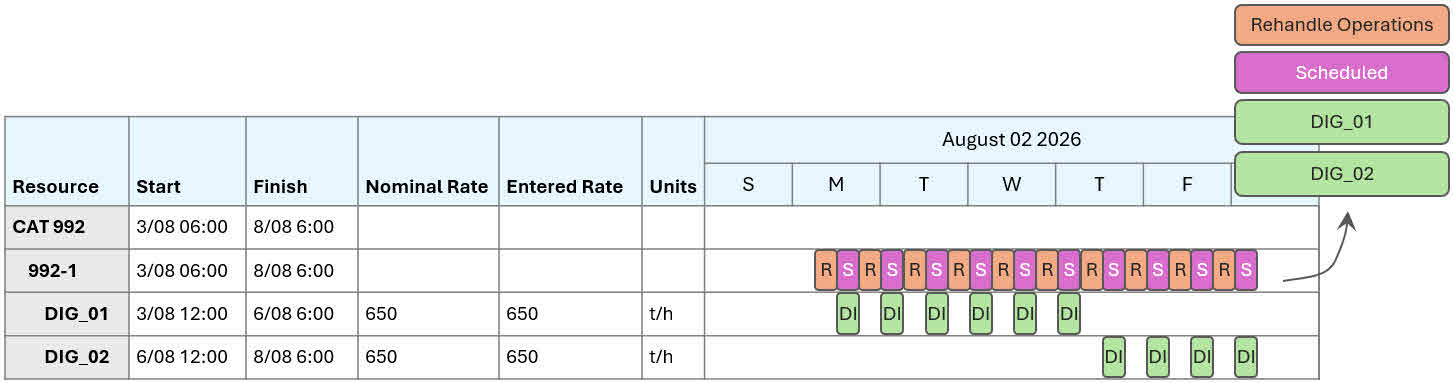
These reductions are reflected in the Gantt chart.

• The actual production rate of the resource within a period reflects these dynamic changes.

• If a resource is delayed, a task labelled Optimiser Delay is inserted into the resource’s row.

Minimum production

Each resource includes a Minimum Production Rate field (refer to Client > Gantt Chart), defined as a factor between 0 and 1 (e.g., 0.5 means the resource can be slowed to 50% of its maximum rate across the period). This factor can vary by resource and period.

Example

If a resource has:

• A base production rate of 1,000 t/h across all periods

• A minimum production rate factor of 0.5

The optimiser can reduce its rate to 500 t/h during periods where slowing production helps meet blend targets.

Rehandle groups

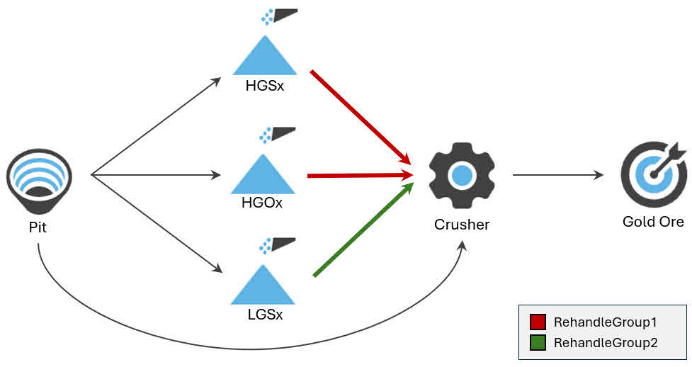
Rehandle groups allow you to model the physical rehandle of material from a stockpile to another location using actual resources like loaders or conveyors. While the Product Optimiser (PO) determines optimal flows based on blending and quality targets, these flows are virtual by default. Rehandle groups bridge this gap by linking physical resources to specific material movements, providing accurate planning and reporting.

What are rehandle groups?

A rehandle group represents a set of material movements (arcs) between a stockpile and another intermediate or a final location (e.g., stockpile → crusher). These groups are defined in the Material flow diagram and are used to associate physical resources with specific rehandling tasks.

Assign resources to rehandle groups

A resource can perform rehandling on a rehandle group’s movements. To set this up, allocate the resource to the Rehandle Operations activity. This activity is system-defined and configured in System Config > Resources.

Each rehandle resource has time usage fields (refer to Client > Resources) that define how much of the resource’s available operating time can be allocated to each rehandle group per period.

• A resource’s total allocation across all rehandle groups must be 0% or 100% per period.

• The schedule uses these allocations to determine how much material each resource can move per group per period.

• Differences in available time (e.g., due to rosters or delays) affect a resource’s total available operating time.

• Resources cannot perform in-pit and rehandle group activities in the same period, but they can switch between them across periods.

Rehandle contribution

Each resource’s contribution to a rehandle group is based on:

• Its rehandle rate (tonnes/hour)

• Its percentage allocation to the group

• Its available operating hours (based on shift length, availability, and utilisation)

These values determine how much material the resource can move in a given period.

Example scenario

Rehandle groups

A site has the following rehandle groups:

Resources

The site has the following resources:

Resource allocation per period

The resources have the following rehandle allocation percentages (defined in Client > Resources). These allocations are the same across each period.

For each resource:

• The maximum amount of time that can be spent operating on a rehandle group is shown.

  • This is calculated by getting the % Time percentage of the resource’s available operating time (11.5 hours).

• The maximum amount of moved material is also shown.

  • This is calculated by taking the available operating time and multiplying it by the resource’s hourly production rate.

Stockpile inventories at start of period

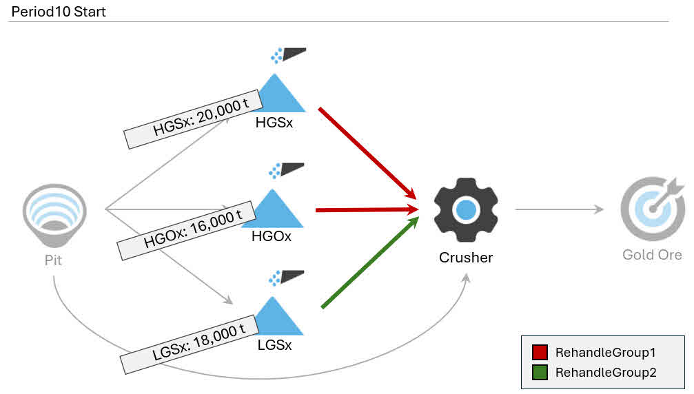
The stockpile inventories at the start of Period 10 are shown below.

Scheduling logic

To allocate resources, the schedule respects the resource limits (refer to Resource allocation per period above) per group:

• Group1: Resource1 (5,520 t) + Resource2 (9,200 t) = 14,720 t (max moved per period)

• Group2: Resource1 only = 3,680 t (max moved per period)

Example allocation

The Product Optimiser attempts to get only one resource to mine from a given stockpile at a time. Before another resource can mine from a stockpile, the other resource must exhaust its capacity on the stockpile within the period. This isn’t always possible – but it’s the likely allocation scenario.

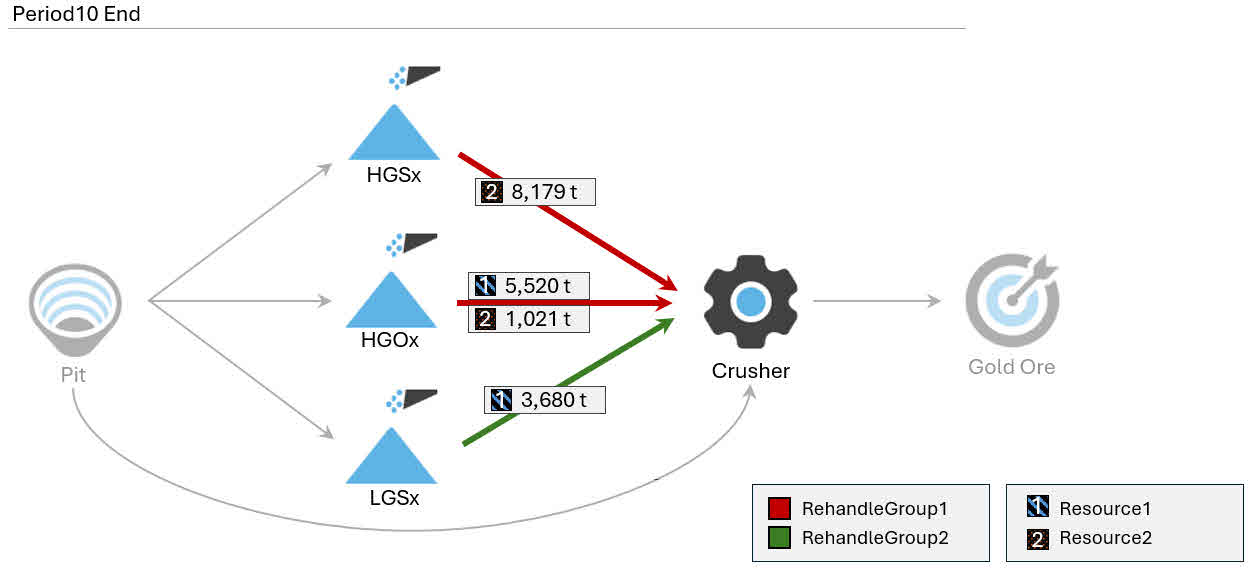
A possible allocation plan for rehandling in Period 10, based on the logic and constraints, is shown below.

1. Resource2 rehandles all tonnes from Group1’s contribution to HGSx (8,179 t).

2. Resource2 then rehandles some of Group1’s contribution to HGOx (1,021 t).

   • The resource’s periodic capacity (800 t/h × 12hrs = 9,600 t capacity) prevents the resource from rehandling more of HGOx.

3. Resource1 then mines as much as it can from HGOx, following its Group1 contribution (5,520 t)

4. Resource1 then mines as much as it can from LGSx, following its Group2 contribution (3,680 t).

The list of rehandling tasks performed within this scenario in Period10

The stockpile inventories and movements in Period10

The distribution of resources across stockpiles within a group may vary depending on scheduling logic. This example shows one valid allocation that meets all constraints.

Rehandle production rate

The production rate of a rehandle resource is set in System Config > Resources.

Rehandle capacity (unlimited or limited)

Each rehandle group can have an unlimited or limited capacity.

Limited capacity

When enabled, the schedule applies a constraint to each rehandle group that limits how much material can be moved across its movements (arcs) in each period. This limit is calculated based on the combined capabilities of the resources assigned to the group.

For each resource, the system considers:

• Its rehandle rate (tonnes per hour)

• The percentage of its time allocated to the group

• Its available operating hours (based on shift length and time usage fields)

These values are used to calculate how much material each resource can contribute to the group in a given period. The total group capacity is the sum of these contributions. The schedule ensures that the total material moved within the group doesn’t exceed this calculated limit.

Unlimited capacity

No constraints are applied, allowing unrestricted movement across the group’s arcs during scheduling.

If the material moved across the rehandle group exceeds the amount that the resources can handle, the schedule increases the resources’ production rates to accommodate all the material. A schedule warning flags this.

Rehandle group processing logic

• Resources obey roster breaks and exceptions.

• Resources try to continue the same task from the end of the previous period into the start of the next to minimise unnecessary movement.

• Reclaiming from staged stockpiles respects:

  • LIFO order (if applicable)

  • Maximum number of concurrent reclaiming piles

  • Reclaim swapping penalties (start, middle, end of period)

• Rehandle groups don’t enforce:

  • Staged stockpile filling limits

  • Instantaneous reclaim rate limits (only total per period)

Rehandle group limitations

• Arcs can belong to only one rehandle group.

• Rehandle groups can only include arcs from stockpiles or staged stockpiles.

• Resources can’t be assigned to both in-pit and rehandle activities in the same period.

Gantt chart visualisation

Rehandle resources are displayed on the Gantt chart (see Gantt Chart) like any other resource. When these resources perform rehandling tasks, a Rehandle Operation bar is shown to indicate the activity. These rehandling delays are non-adjustable directly on the chart.

You can assign in-pit activities to rehandle resources, provided those resources are permitted to perform such tasks.

Reporting Gantt chart

You can build custom reports (refer to Reporting tab) and Gantt charts (refer to Gantt Reporting tab) to see the full detail of each material movement assigned to a rehandle group, such as the:

• Source and destination of each movement

• Quantities and qualities of materials

• Rehandle group names and associated tasks

Visualise multiple operations

Custom Gantt charts can integrate rehandle tasks with other operational schedules, such as in-pit mining, plant maintenance, and train logistics. This unified view helps identify dependencies and optimise coordination across different activities.

For example, a custom Gantt chart could display:

• The sequence of rehandle tasks across each period

• Locations (e.g., stockpiles) as primary visual elements

• Resources such as fixed plant, mobile equipment, and other machinery

• Interdependencies between schedules (e.g., how plant maintenance affects train operations, train allocations to specific stockpiles)

• Live and dead stockpile locations

For staged stockpiles, the report can display detailed build sequences, including stacking and reclaiming start and finish times. These tasks provide a complete picture of stockpile activity alongside rehandling operations.